Module 2 Feldspar reaction path

In this tutorial, you will learn to model the reaction path of K-feldspar in contact with a NaCl-bearing aqueous solution and calculate the evolution of the fluid and the minerals formed as a function of increased fluid-rock interaction. You will also learn how to set up an automated cooling process simulation and plot results from multiple simulations. We will use the GEMS project file “Module2” that can be found either in the /Tutorial/Module2 workshop folder or download it directly here.

2.1 Compute the chemical equilibrium of single chemical systems (SysEq)

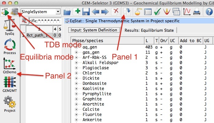
Figure 2.1: GEMS user interface showing the Equilibria Calculation and Thermodynamic Database modes.

• Copy the entire unzipped Module2 folder into your GEMS project directory located in Library/Gems3/projects. More information on the GEMS folder structure can be found in Module 1.

– For Windows users the project folder is located in C:/GEMS370/Library/Gems3/projects/ or similar.

– For Mac OSX users, open Finder, on the top click on Go to… and enter ~/Library/Gems3

• Open GEMS and choose the project in the Equilibria Calculation Mode. The user interface is shown in Figure 2.1. Panel 1 permits to create new records and run the program for calculations. Panel 2 gives you different calculation options.

• Choose the Create a new record from scratch from the menu in Panel 1 and fill the parameters listed in Figure 2.2

• In the Open recipe dialog, which can also be found in Panel 1, add phases, quantity and units as shown in Figure 2.3; Aqua (1000 g), HCl (0.1 M), NaCl (50 g), O\(_{2(g)}\) (1e-7) and K-feldspar (10 g).

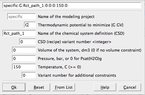
Figure 2.2: New record window. Select a name without spaces, a temperature and a pressure for your system. Note that a pressure of 0 corresond to saturated water vapor pressure.

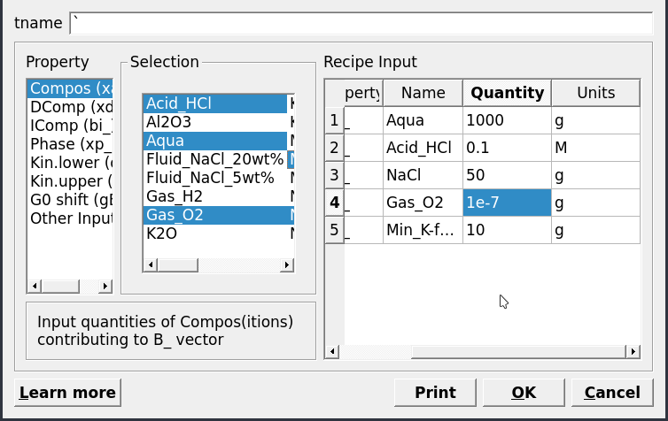
Figure 2.3: System recipe dialog.

• Model the chemical equilibrium between 10 g of K-feldspar (microcline) and H\(_2\)O at 150 \(^\circ\)C by pressing Calculate BCC followed by Calculate Equilibrium in Panel 1. Inspect the pop up window with pH, redox (eH) and phase proportions, then accept.

  – Determine the pH of this system as shown in the lower right of the main window (Fig. 2.4).

  – What is the pH of this system with 10, 20, 50 and 100 g K-feldspar? Change the amount of feldspar by clicking the Open recipe dialog followed by Calculate BCC and by Calculate Equilibrium. What minerals are stable with increasing pH?

• Finally, clone your existing Rct_path_1 chemical system by selecting it and choosing Clone a new record from this one in Panel 1 (Fig. 2.1). Change the name to Rct_path_2 and the temperature to 300 \(^\circ\)C in the pop up window, and recalculate the equilibrium of this system.

  – Determine the pH of this system as shown in the lower right of the main window.

  – What is the pH of this system with 10, 20, 50 and 100 g K-feldspar? What minerals are stable with increasing pH?

  – Are there differences between the modeled system at 150 and 300 \(^\circ\)C

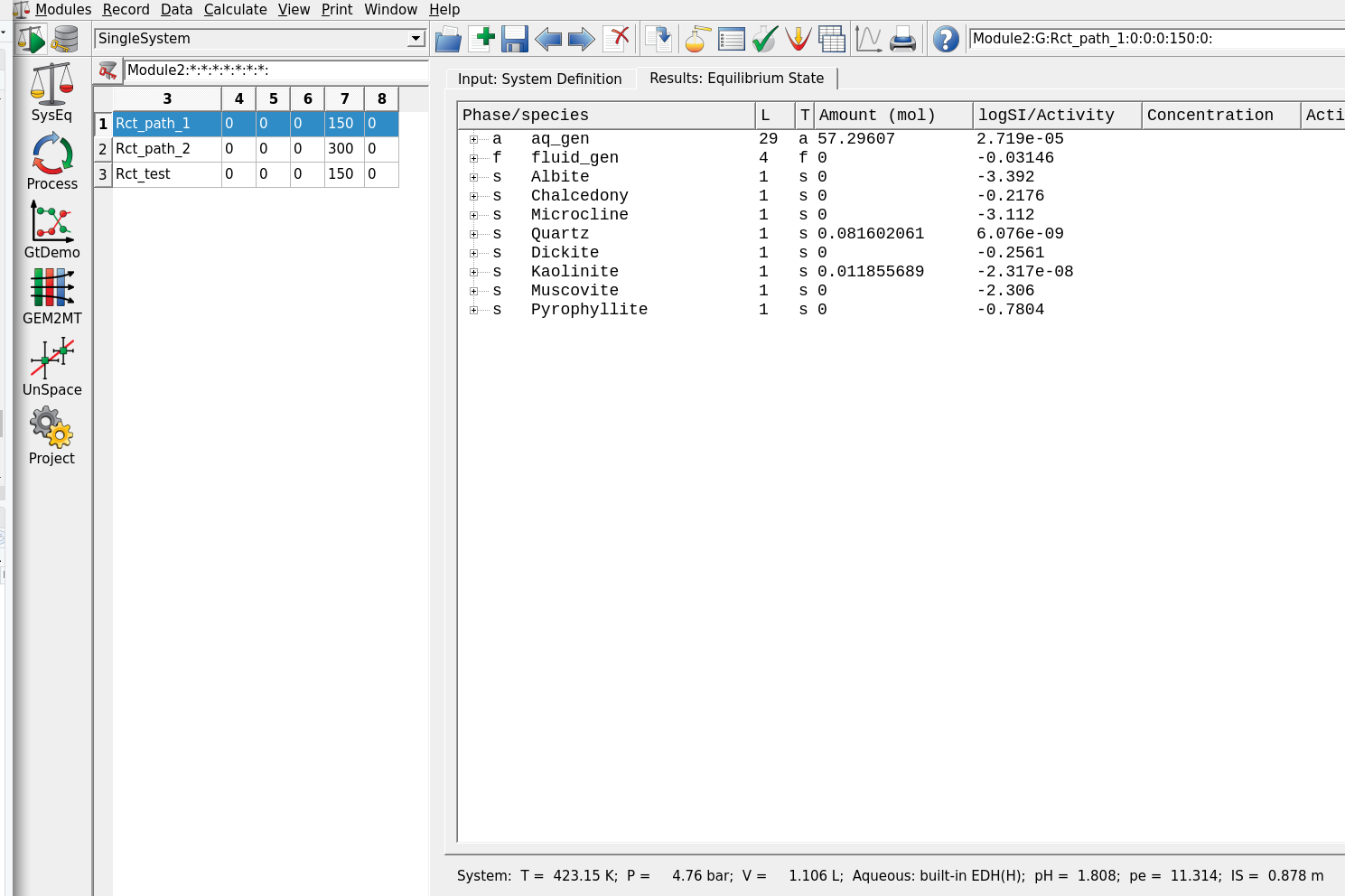
Figure 2.4: Results of the calculations, i.e. with 10 g K-feldspar added to the fluid.

2.2 Compute a titration model (Process, S mode)

The previous part of this tutorial showed you how to do individual SysEq calculations. What if you want to automate this process and calculate the equilibria of 10 to 100 g feldspar in steps and plot the results, i.e. a titration model? In the following we will see how to set up Process simulations.

• Select the Process option in Panel 2 (Fig. 2.1).

• Click Create a record from scratch in Panel 1 and select your parent chemical system SysEq calculated previously at 150 \(^\circ\)C (Fig. 2.5).

• Name this process simulation “titration_150C” and use the Process simulation code (S) as shown in Figures 2.6) and 2.7).

• In the next window, choose a model (titration cNu linear), a mineral ( Compos, Min_K-feldspar) and select the temperature (150 \(^\circ\)C), pressure (0 for water vapor saturation P) and amount of mineral to be added (iNu: 10-250 g in 10 g steps) as shown in Figure 2.8. The parameters are: set iTm 1000, 1200, 1; set iP to 0 all fields; set iNu 10, 250, 10, corresponding to start, end, and step values.

• Select items to be plotted (Scalars: pH; Xa: Kaolinite, Pyrophyllite, Microcline, Muscovite, Albite and Quartz) as shown in Figure 2.9.

• Accept all the following dialogues. Then click on Save this record to database in Panel 1, which creates your new process simulation record. Then click on the calculator icon Re-calculate and check record data without displaying the graph.

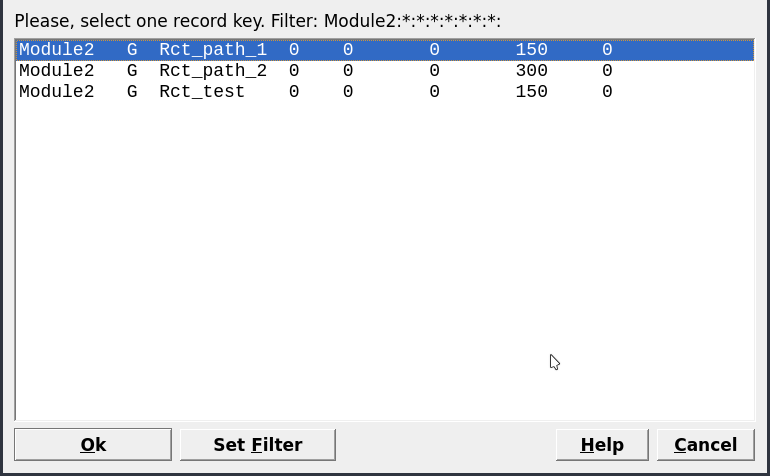
Figure 2.5: Select a parent chemical system (SysEq) for modeling a Process.

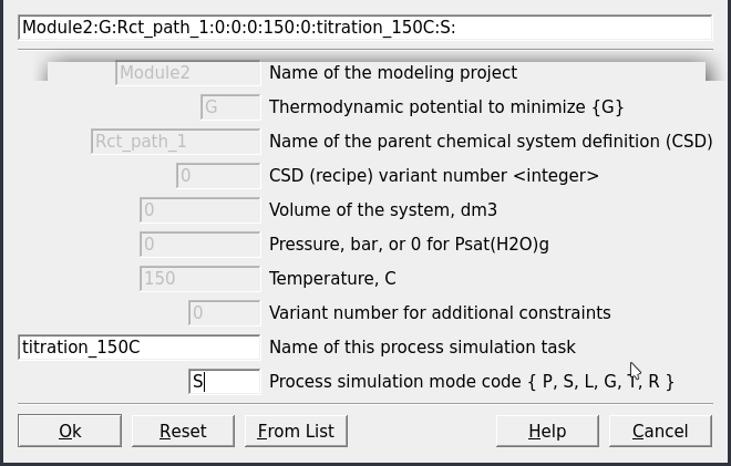
Figure 2.6: Name the Process simulator and indicate the model type (note: the process type code names are described and changeable on the next screen as well).

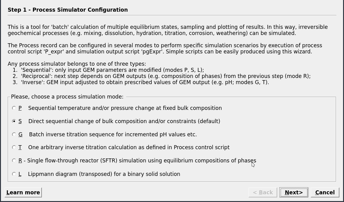
Figure 2.7: Window showing the different simulations types. Module 2 covers mode S for titration or mode P for cooling/heating models.

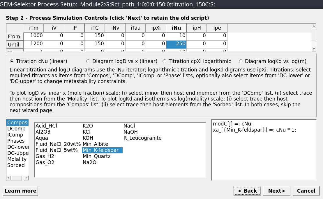
Figure 2.8: Set the parameters for the Process simulation; Set iTm 1000, 1200, 1; Set iP to 0 all fields; Set iNu 10, 250, 10.

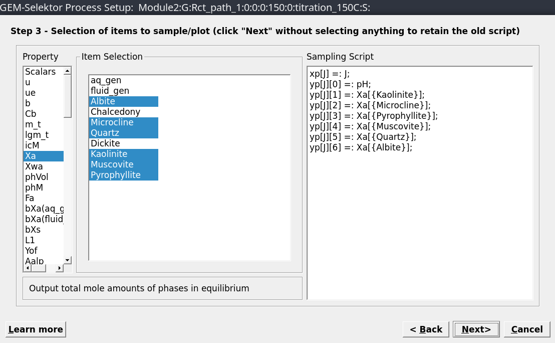
Figure 2.9: Choose the results to be plotted, including pH and mole minerals.

• There is a tab menu with 3 important selections: Controls, Sampling and Results. In the Controls tab add a description of the modeling project (Fig. 2.10). In the Sampling tab change the script as shown in Figure 2.11 to choose as x-variable the amount of K-feldspar added (the process extent variable cNu).

• Click Save this record to database. Toggle to the Results tab to inspect your modeling results. Then click on the calculator icon Re-calculate and check record data and check what happens with the column xp. You just assigned the cNu variable to the x-axis and GEMS registered it. If not, go back on the Sampling tab and check your script! Now lets inspect the results…

  – How many grams of K-feldspar need to be added to get a constant pH and what is the value?

  – Which mineral assemblages buffer the fluid pH and can pH ranges be distinguished?

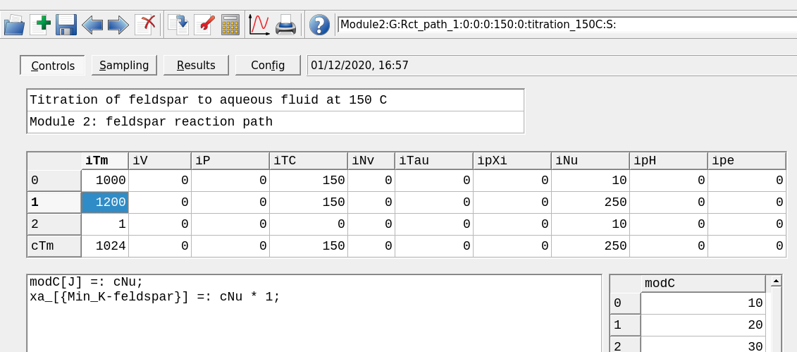
Figure 2.10: The Controls window showing the model conditions. The top dialog is used to add a comment and the script dialog can be customized. iTm is used to set the record variable; iP to set pressure and iTC temperature; iNu is the process variable, in this case the amount of feldspar.

Figure 2.11: The Sampling window showing the x- and y-axes to be sampled. Make sure to change xp[J] to cNu which is the progress variable. Then click on a blank space to make sure the script window has been registered followed by Save this record in the database in the top panel.

2.3 Modify P-T of the feldspar reaction path

Now lets clone our record to calculate the exact same titration model but changing the temperature (T) to 300 \(^\circ\)C and the pressure (P) to 500 bar.

• Clone your existing process simulation by selecting the existing record on the left and choose Clone a new record, then select your SysEq parent system calculated at 300 \(^\circ\)C (Fig. 2.12). Accept all the following dialogues.

• In the Controls tab change the description of the modeling project and change the temperature to 300 \(^\circ\)C and pressure to 500 bar to replace the starting and ending values (Fig. 2.13). Click Save this record to database.

• Switch the tab to Results and click the calculator icon Re-calculate and check record data to see how the pH values and moles minerals are changed by increasing the system temperature.

• Toggle between both calculated process simulations at 150 and 300 \(^\circ\)C on the left pane and compare the results.

Figure 2.12: The Sampling window showing the x- and y-axes to be sampled. Make sure to change xp[J] to cNu which is the progress variable. Then click on a blank space to make sure the script window has been registered followed by Save this record in the database in the top panel.

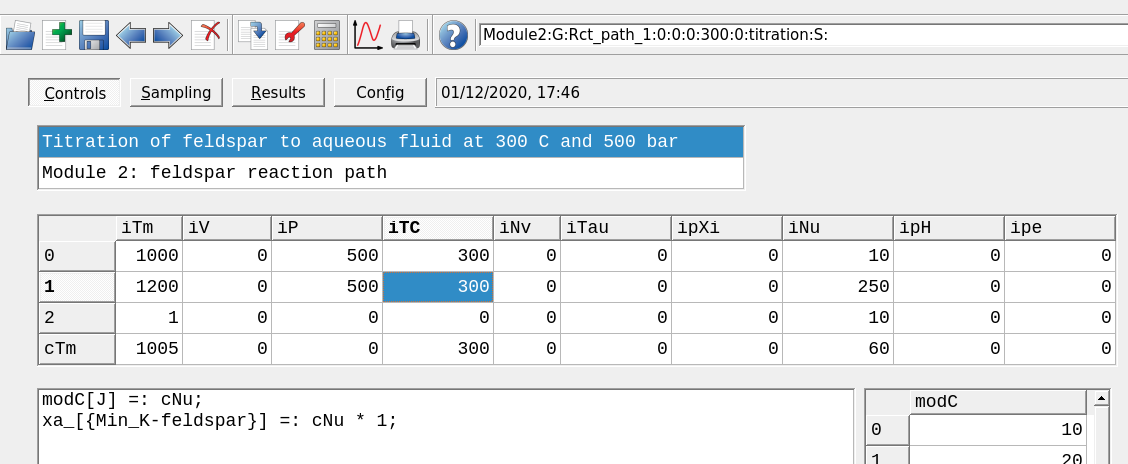
Figure 2.13: The Controls window showing a model set up at a different temperture and pressure.

2.4 Tweak and plot the results

So what are the main differences for the simulations at 150 vs. 300 \(^\circ\)C? To make a better comparison lets fine tune our models and plot them!

• Select the process simulation you generated previously at 150 \(^\circ\)C and in the Controls tab change the amount of K-feldspar to be added using 2 to 50 g in 2 g steps and save.

• Choose the Results tab and click the calculator icon Re-calculate and check record data. Click on the small Plot data on Graph dialog icon in Panel 1. The resulting graph should look similar to Figure 2.14. The plots indicate that different mineral assemblages buffer the fluid pH values.

• You can inspect which minerals by clicking the Customize button at the bottom of the plot and enter the values shown in 2.15, then click Apply. Click then on Fragment which will enable an inset view of your plot to have a closer look at the minerals. Clicking again Fragment zooms out to show the pH. It is also possible to do this with the mouse, but note that this will then overwrite the x-y-axis ranges you just entered manually.

• To label the lines on the plot simply drag the mineral names from the legend on the right into your plot.

• You can also switch on/off minerals or pH by toggling the corresponding fields in the laegend from 0 to off (or o-letter or 0-number keys on your keyboard). Now you should be able to reproduce the look in Figure 2.14. To save, simply click on Save at the bottom of your plot in the desired format (e.g. pdf, png, etc.).

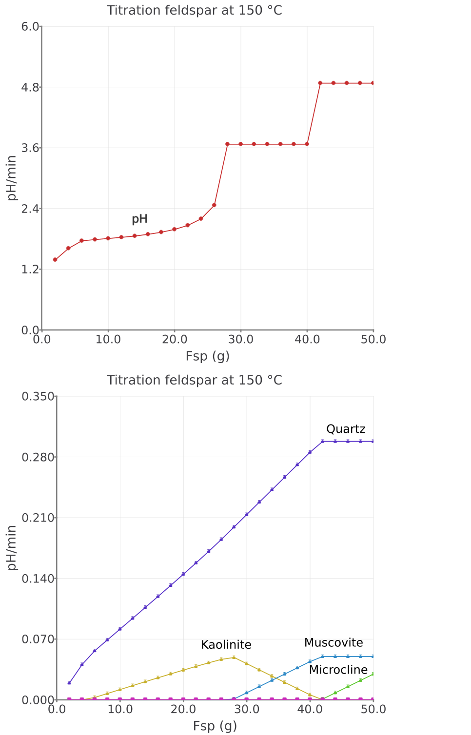
Figure 2.14: Simulated K-feldspar reaction path show pH and moles minerals in equilibrium with a saline aqueous fluid at 150 °C and saturated water vapor pressure.

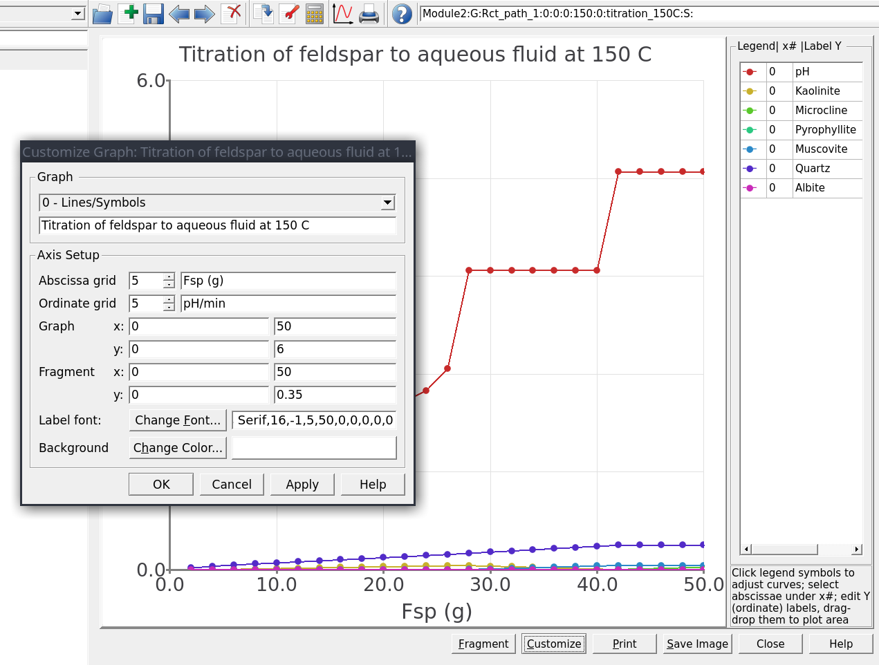
Figure 2.15: Customize window showing options to tweak the plot. Here you can change the plot type, x- and y-axes, the font size, add labels and also the zoom-in feature by selecting x-y under Fragment. The right legend can also be turned on/off by toggling 0 to off (or using the o-letter or 0-number keys on your keyboard), and legend names dragged into the plot.

• Now select the process simulation you generated previously at 300 \(^\circ\)C and 500 bar. In the Controls tab change the amount of K-feldspar to be added using 5 to 125 g in 5 g steps, re-calculate and save. Try to tweak your graph to look like Figure 2.16.

• Figure 2.17 shows an alternative way to make a cumulative plot.

• You can now easily compare both feldspar reaction path models generated using the Process simulation in S mode!

– The resulting reaction path at 150 \(^\circ\)C is shown in Figure 2.14.

– The resulting reaction path at 300 \(^\circ\)C is shown in Figure 2.16.

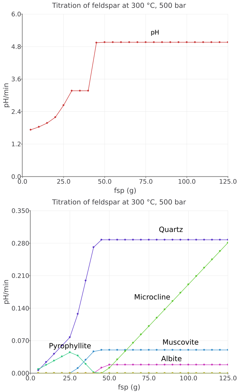
Figure 2.16: Simulated K-feldspar reaction path show pH and moles minerals in equilibrium with a saline aqueous fluid at 300 °C and 500 bar.

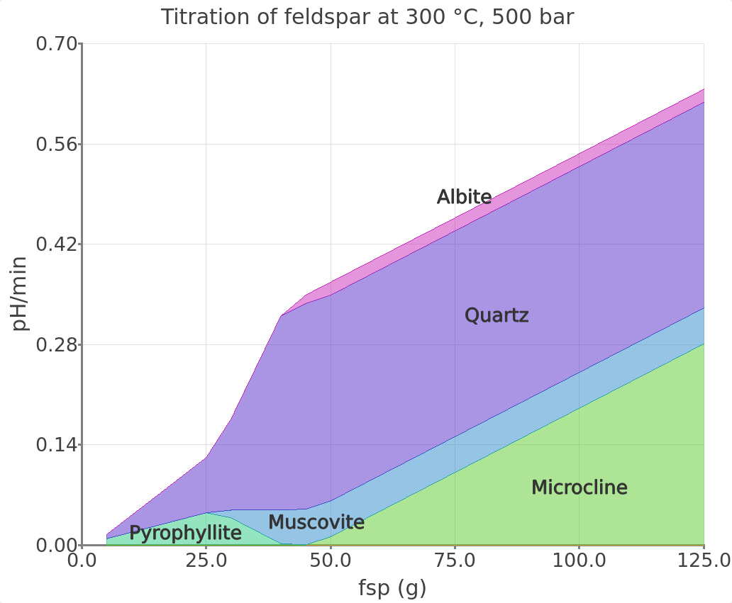
Figure 2.17: Simulated K-feldspar reaction path show pH and moles minerals in equilibrium with a saline aqueous fluid at 300 °C and 500 bar. To view this plot type choose the option 1- Cumulative plot in the plot Customize window. Make sure to also switch off pH in the legend to only plot moles minerals.

2.5 Compute a cooling model (Process, P mode)

This part of Module 2 describes how to calculate the equilibrium between feldspar and the aqueous fluid at a constant mineral/fluid ratio but varying temperature. We will set up a cooling model from 150 to 300 \(^\circ\)C in selected steps using the Process simulation in P mode. We will use knowledge gained until here. This part is quick so buckle up!

• Create a parent system equilibrium record in SysEq simulation mode 2.4 by cloning Rct_path_2. Lets call this new record Rct_cooling, select 300 °C and 500 bar, and calculate its equilibrium.

• Switch to Processsimulation mode and clone Rct_path_2. Select the Rct_cooling SysEq record (Fig. 2.18). Then call this new record Cooling_150-300C and select P for the simulation mode.

• In the Controls tab (or wizard step 2) select No script, set iNu to 0 and iTC to 300, 150, -5 as shown in Figure 2.19.

• The final step is to set the x-variable to temperature by modifying the script in the Sampling tab to cTC (Fig. 2.20). Save your record and re-calculate.

• Now you can plot and tweak your results to look similar to Figure 2.21).

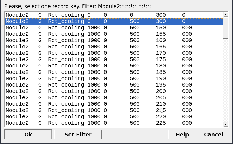
Figure 2.18: Select the parent record generated in SysEq for your new Process simulation.

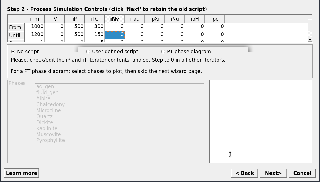
Figure 2.19: Controls window showing the set up for a cooling model (no titration); select No script, set iNu to 0 and iTC to 300, 150, -5.

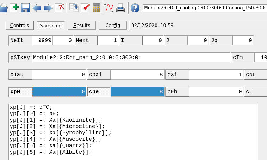
Figure 2.20: Sampling tab window showing how to modify the x-axis to display temperature cTC.

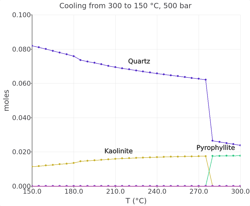
Figure 2.21: Cooling model showing the feldspar reaction path between 300 and 150 °C in 5 °C steps at a fluid/rock ratio of 100.

2.6 Outcomes

Good job! In Module 2 you learned how to run and automate fluid-mineral equilibria simulations using the Process mode. You can now generate titration models in S mode or cooling models in P mode. You also know how to do plots in GEMS, tweak and export them.